Machine learning - Lundquist Urban Ecology Lab

Machine learning is a subfield of artificial intelligence that involves the development of algorithms and models that can learn from and make predictions or decisions based on data. There are many different types of machine learning algorithms, each with their own strengths and weaknesses, and they can be applied to a wide variety of problems.

Decision trees

One of the most popular and widely used types of machine learning algorithms is decision trees. Decision trees are a type of algorithm that can be used for both classification and regression problems. They work by recursively partitioning the data into subsets based on the values of the input features, and making predictions based on the majority class or mean value of the observations in each subset.

Here’s an example of how decision trees can be implemented in R:

	library(rpart)

	# Load data
	data <- iris

	# Build decision tree
	fit <- rpart(Species ~ Sepal.Length + Sepal.Width + Petal.Length + Petal.Width, data = data, method = "class")

	# Plot the decision tree
	library(rpart.plot)
	rpart.plot(fit)

view raw decision_tree.r hosted with ❤ by GitHub

R code

rpart.plot output for decision trees using Iris dataset

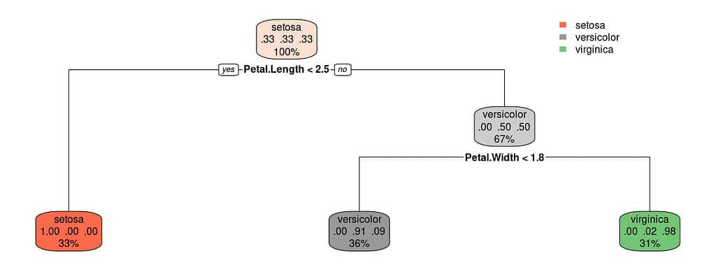
In this example, we are using the iris dataset, a popular dataset for classification problems that contains measurements of sepals and petals of three different species of irises. We are using all the columns as predictors and the species as response. The rpart function is used to build the decision tree model, and the rpart.plot is used to plot the tree.

We can do the same thing in Python:

	from sklearn.tree import DecisionTreeClassifier
	from sklearn.datasets import load_iris
	from sklearn.model_selection import train_test_split

	# Load data
	iris = load_iris()
	X = iris.data
	y = iris.target

	# Split data into training and testing sets
	X_train, X_test, y_train, y_test = train_test_split(X, y, test_size=0.2, random_state=42)

	# Build decision tree
	clf = DecisionTreeClassifier()
	clf.fit(X_train, y_train)

	# Make predictions on the test set
	y_pred = clf.predict(X_test)

	# Evaluate the model's performance
	from sklearn.metrics import accuracy_score
	print(accuracy_score(y_test, y_pred))

view raw decision_tree.py hosted with ❤ by GitHub

Python code

The train_test_split() function is used to split the data into a training set and a test set, the DecisionTreeClassifier() function is used to build the decision tree model and the fit function is used to train the model. The predict function is used to make predictions on the test set, and the accuracy_score() function is used to evaluate the model’s performance by comparing the predicted values to the actual values.

Linear models

Another popular type of machine learning algorithm is linear regression. Linear regression is a type of algorithm that can be used for continuous target variables and it attempts to find the best linear relationship between the input features and the target variable.

Here’s an example of how linear regression can be implemented in R:

	# Load data
	data <- mtcars

	# Build linear regression model
	fit <- lm(mpg ~ wt + hp, data = data)

	# Summarize the model
	summary(fit)

view raw linear_regression_ML.r hosted with ❤ by GitHub

R code

In this example, we are using the mtcars dataset, a dataset that contains measurements of different cars such as the miles per gallon, weight, and horsepower. We are using the weight and horsepower as predictors and the miles per gallon as the target variable. The lm() function is used to build the linear regression model and the summary function is used to summarize the model.

We can also run linear regressions in Python:

	import pandas as pd
	from sklearn.linear_model import LinearRegression
	from sklearn.model_selection import train_test_split

	# Load data
	url = 'https://gist.githubusercontent.com/ZeccaLehn/4e06d2575eb9589dbe8c365d61cb056c/raw/898a40b035f7c951579041aecbfb2149331fa9f6/mtcars.csv'
	data = pd.read_csv(url, index_col=0)
	print(data.head(5))


	data = pd.read_csv("data.csv")

	# Split data into training and testing sets
	X_train, X_test, y_train, y_test = train_test_split(data[['wt','hp']], data['mpg'], test_size=0.2, random_state=42)

	# Build linear regression model
	reg = LinearRegression()
	reg.fit(X_train, y_train)

	# Make predictions on the test set
	y_pred = reg.predict(X_test)

	# Evaluate the model's performance
	from sklearn.metrics import mean_squared_error
	print(mean_squared_error(y_test, y_pred))

view raw linear_regression_ML.py hosted with ❤ by GitHub

Python code

In this example, we are using the mtcars dataset from this Gist. The predictors are the weight and horsepower and the target variable is the miles per gallon. The train_test_split() function is used to split the data into a training set and a test set, the LinearRegression() function is used to build the linear regression model, and the fit function is used to train the model. The predict function is used to make predictions on the test set, and the mean_squared_error() function is used to evaluate the model’s performance by comparing the predicted values to the actual values.

Artificial neural networks (ANNs)

Finally, another popular type of machine learning algorithm is artificial neural networks (ANNs). Artificial neural networks are a type of algorithm that are inspired by the structure and function of the human brain. They are composed of layers of interconnected “neurons” that process and transmit information. They are highly flexible and can be used for a wide variety of problems, including image and speech recognition, natural language processing, and more.

Here’s an example of how ANNs can be implemented in R using the caret package:

	# Load data
	data <- iris

	# Split data into training and testing sets
	set.seed(123)
	index <- sample(1:nrow(data), 0.8 * nrow(data))
	train <- data[index,]
	test <- data[-index,]

	# Build ANN model
	library(caret)
	model <- train(Species ~ ., data = train, method = "mlp", trControl = trainControl(method = "cv", number = 5))

	# Make predictions on the test set
	predictions <- predict(model, newdata = test)

	# Evaluate the model's performance
	confusionMatrix(predictions, test$Species)

view raw ANN.r hosted with ❤ by GitHub

R code

In this example, we are again using the iris dataset, but this time we are splitting the data into a training set and a test set. We are using all the columns as predictors and the species as response. The train function is used to build the ANN model, specifying the “mlp” method for neural networks, and using k-fold cross validation with k=5 to train the model. The predict function is used to make predictions on the test set, and the confusionMatrix() function is used to evaluate the model’s performance by comparing the predicted values to the actual values.

In Python:

	from sklearn.neural_network import MLPClassifier
	from sklearn.datasets import load_iris
	from sklearn.model_selection import train_test_split

	# Load data
	iris = load_iris()
	X = iris.data
	y = iris.target

	# Split data into training and testing sets
	X_train, X_test, y_train, y_test = train_test_split(X, y, test_size=0.2, random_state=42)

	# Build ANN model
	clf = MLPClassifier(hidden_layer_sizes=(10,),max_iter=1000)
	clf.fit(X_train, y_train)

	# Make predictions on the test set
	y_pred = clf.predict(X_test)

	# Evaluate the model's performance
	from sklearn.metrics import accuracy_score
	print(accuracy_score(y_test, y_pred))

view raw ANN.py hosted with ❤ by GitHub

Python code

This example again uses the iris dataset. We are using all the columns as predictors and the species as response. The train_test_split() function is used to split the data into a training set and a test set, the MLPClassifier() function is used to build the ANN model, the fit function is used to train the model, the predict function is used to make predictions on the test set, and the accuracy_score() function is used to evaluate the model’s performance by comparing the predicted values to the actual values.

Machine learning is a powerful tool that can be used to extract insights from data and make predictions and decisions. There are many different types of machine learning algorithms, each with their own strengths and weaknesses, including decision trees, linear regression, and artificial neural networks. These examples in R demonstrate how to implement these algorithms, but it’s important to note that the performance of these models may vary depending on the specific problem and the quality of the data. It’s also important to understand the underlying concepts of each algorithm and the assumptions they make, to make the right choice for a given problem.