Predicting the future
Before this point, we have been using statistics to compare groups of observations and determining the probability that the differences we see between groups is no due to random chance. However, the real strength of statistics is the ability to use probability and current observations to predict future observations and trends. The basic way we can do this is through correlation and regression of two continuous variables.
Correlation
A correlation is a determination about how well we can predict y (dependent variable) from x (independent variable). The parameter for a correlation is ρ and the estimate is r.
A correlation is performed by measuring covariance.
- Covariance is how two observations measured from the same subject deviate together from their means.
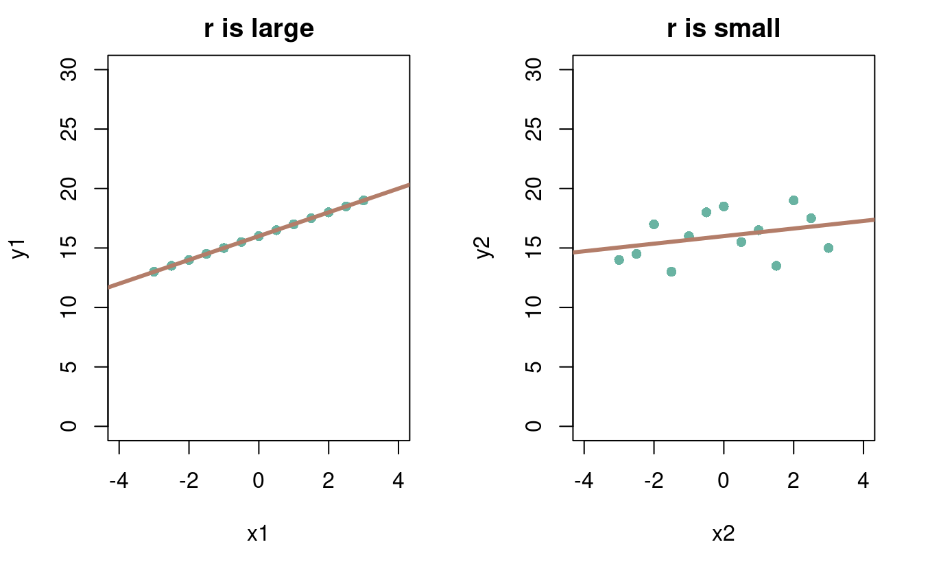
- r describes how reliably x and y change together. We call r the correlation coefficient.
- R² describes the amount of variation in one variable that can be predicted from the other (see ANOVA)


Assumptions:
- x is normal with equal vars for all values of y
- y is normal with equal vars for all values of x
- Relationship between x and y is monotonoic (i.e. rise or fall together)
Note: a significant correlation does not equal causation. It is up to the statistician to think critically about the relationships between the two sets of data.
Regression
A regression is how the expectation of y changes with a change in x. The parameter is β and the estimate is b. You may have heard of regression as the “line of best fit”.
- a = intercept
(prediction y for x = 0) - b = slope
(unit increase y for increase y)


Assumptions:
- Samples are random
- y is normally distributed with variance independent of x
- The relationship between x and y can be described as a line
Note: x does not have to be normally distributed