Analysis of variance - Lundquist Urban Ecology Lab

Comparing means of more than two groups

We can use the analysis of variance (ANOVA) is a special type of non-parametric test used to compare means between normally distributed populations from more than groups.

ANOVA basics

Assumptions:

Samples are taken randomly
Measurements from each population is normally distributed
The variances are equal between all populations

MS_groups: mean square of groups

MS_error: mean square of error

Calculating the ANOVA test statistic

Step 1: Partition the sum of squares

Calculate a grand mean by taking the sum of the product of the means and sample size of each group divided by the N total number of observations.

Sum of squares of the groups

Sum of squares of the error

Step 2: Calculate the mean squares

Mean square groups

Mean square error

k = number of groups

Step 3: Build ANOVA table

Source of variance	Sum of squares	df	Mean squares	F	P
Groups	SS_groups	groups – 1	MS_groups	MS_groups / MS_error	P-value
Error	SS_error	observations – groups	MS_error
Total	SS_total	df_error + df_groups

Step 4: If the null is rejected, perform a post-hoc test to determine differences between groups

This can be done using a Tukey-Kramer test

Determining the variance explained by differences in groups

Checking assumptions

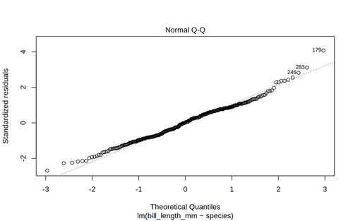
The normality assumption can be checked visually by looking at a Q-Q plot of the residuals. If the points fit the straight line well, we can claim that they are normally distributed.

Homogeneity of variances can be checked either by using a Levene’s test or Bartlett’s test.

	data(iris)
	df <- iris

	# Box plots
	boxplot(Petal.Width ~ Species, data = df)

	# Strip plot
	library(lattice)
	stripplot(Petal.Width ~ Species, data = df, jitter = TRUE)

	# ANOVA
	model <- lm(Petal.Width ~ Species, data = df)
	summary(aov(model))
	# OR
	anova(model)

	# Tukey HSD
	TukeyHSD(aov(model))

	# Check assumptions
	par(mfrow = c(2, 2))
	plot(model) ## QQ plots and others

	# Shapiro-Wilk test for normality
	shapiro.test(df$Petal.Width)

	# Bartlett test for homogenety of variances
	bartlett.test(Petal.Width ~ Species, data = df)

	# Levene's test for homogeneity of variances
	library(car)
	leveneTest(Petal.Width ~ Species, data = df)

view raw anova.r hosted with ❤ by GitHub

R code

	import pandas as pd
	import scipy.stats as stats
	import matplotlib.pyplot as plt
	import seaborn as sns
	import statsmodels.api as sm

	from sklearn.datasets import load_iris
	from bioinfokit.analys import stat
	from statsmodels.formula.api import ols

	# Y needs to be continuous and needs to be organized into > two X groups.
	iris = load_iris()

	df = pd.DataFrame(data=iris.data, columns=iris.feature_names)
	df['target'] = iris.target
	df['species'] = df['target'].apply(lambda x: iris.target_names[x])

	print(df)

	# Rename the column of interest so it does not have spaces
	df = df.rename(columns={'petal width (cm)': 'petal_width'})


	ax = sns.boxplot(x='species', y='petal_width', data=df, color="#99c2a2")
	ax = sns.stripplot(x='species', y='petal_width', data=df, color="#7d0013")
	plt.show()

	## Interested in petal width

	setosa = df.loc[df['species'] == "setosa"]
	versicolor = df.loc[df['species'] == "versicolor"]
	virginica = df.loc[df['species'] == "virginica"]


	# For just F and P value
	fvalue, pvalue = stats.f_oneway(setosa['petal_width'], versicolor['petal_width'], virginica['petal_width'])
	print(fvalue, pvalue)


	## ANOVA table
	# Ordinary Least Squares model
	model = ols('petal_width ~ species', data=df).fit()
	anova_table = sm.stats.anova_lm(model, typ=2)
	anova_table

	# Tukey HSD

	res = stat()
	res.tukey_hsd(df=df, res_var='petal_width', xfac_var='species', anova_model='petal_width ~ C(species)')
	res.tukey_summary

	# Check assumptions
	# QQ-plot
	import statsmodels.api as sm
	import matplotlib.pyplot as plt

	sm.qqplot(res.anova_std_residuals, line='45')
	plt.xlabel("Theoretical Quantiles")
	plt.ylabel("Standardized Residuals")
	plt.show()

	# histogram
	plt.hist(res.anova_model_out.resid, bins='auto', histtype='bar', ec='k')
	plt.xlabel("Residuals")
	plt.ylabel('Frequency')
	plt.show()

	# Shapiro-Wilk test for normality
	w, pvalue = stats.shapiro(model.resid)
	print(w, pvalue)

	# Bartlett test for homogeneity of variances
	w, pvalue = stats.bartlett(setosa['petal_width'], versicolor['petal_width'], virginica['petal_width'])
	print(w, pvalue)

	## Levene's test for homogeneity of variances
	res = stat()
	res.levene(df=df, res_var='petal_width', xfac_var='species')
	res.levene_summary

	# It seems that we should be using the non-parametric ANOVA (Kruskal-Wallace)

view raw anova.py hosted with ❤ by GitHub

Python code